
How does a decision tree split data to make predictions?
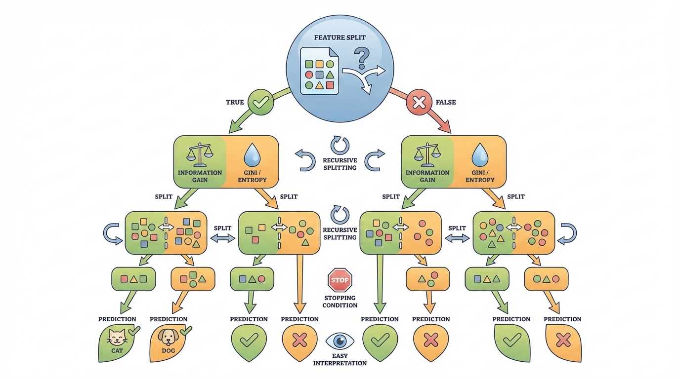
A decision tree is a supervised machine learning algorithm
that makes predictions by repeatedly splitting data based on feature values.
Each split is chosen to best separate the data into meaningful groups.
How a decision tree works:
- Selects the feature that provides the highest information gain or lowest impurity
- Creates internal nodes that represent decision conditions
- Splits the dataset into smaller subsets at each node
- Uses metrics such as Gini impurity or entropy to evaluate splits
- Repeats the process until a stopping condition is met
The final nodes, called leaf nodes, represent the predicted
outcomes. This tree-like structure makes decision trees easy to understand
and interpret.
Real-life example:
In banking, decision trees are commonly used to decide whether a loan should
be approved. The model may check conditions such as income level, credit score,
and employment status step by step, finally reaching a clear “approve” or
“reject” decision that can be easily explained to customers.
Explain how k-means clustering groups unlabeled data.
K-means clustering is an unsupervised machine learning algorithm
used to group data points into clusters based on similarity.
Each cluster is represented by a central point called a centroid.
How the K-means algorithm works:
- Selects K initial centroids randomly
- Assigns each data point to the nearest centroid
- Recalculates centroids as the mean of assigned points
- Repeats assignment and update steps iteratively
- Stops when centroids stabilize or a maximum iteration limit is reached
Key characteristics:
- Final clusters contain data points with similar characteristics
- Performs best with spherical and evenly sized clusters
- Simple, fast, and scalable for large datasets
Real-life example:
In retail analytics, K-means is often used to segment customers based on
purchase behavior. Customers with similar spending patterns are grouped
together, helping businesses design targeted marketing campaigns and
personalized offers.
How does linear regression fit the best line for prediction?
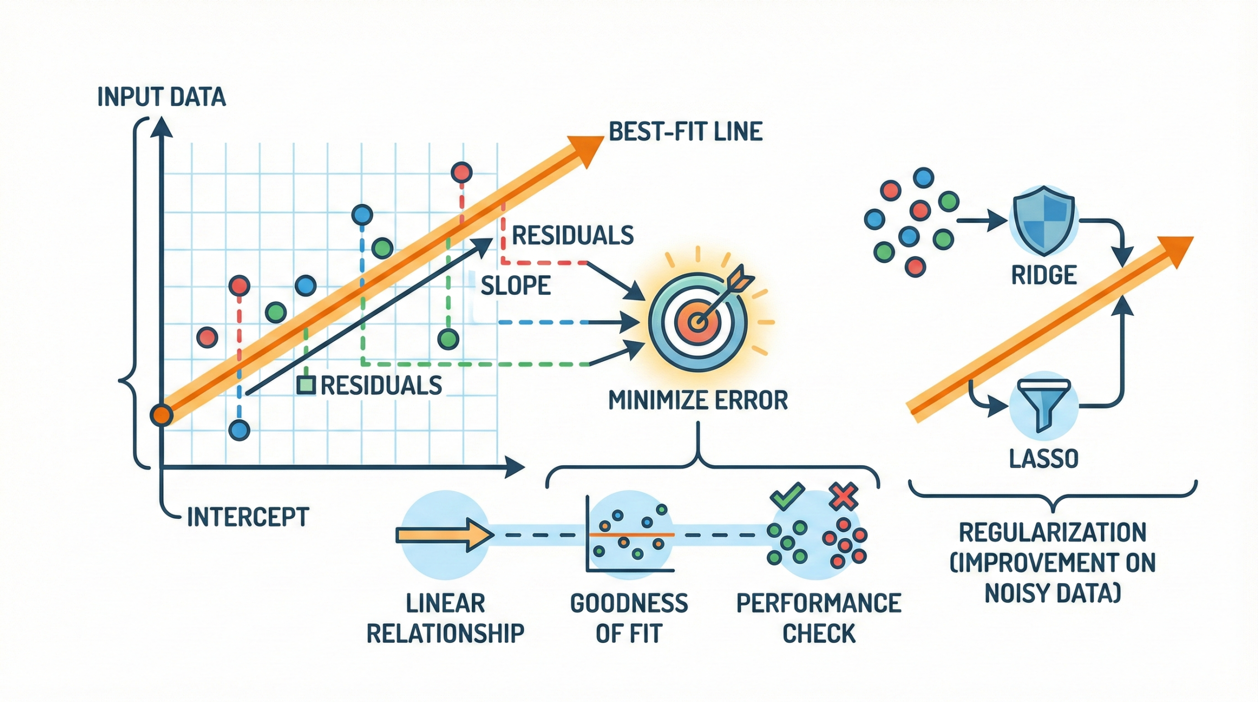
Linear regression is a supervised machine learning algorithm
used to model the relationship between input features and a continuous output
by fitting the best possible straight line through the data.
How linear regression works:
- Finds the optimal line that minimizes the sum of squared residuals
- Calculates the slope and intercept using formulas or optimization methods
- Assumes a linear relationship between inputs and output
- Uses residual plots to evaluate model fit and error patterns
To handle noisy or high-dimensional data, regularized versions such as
Ridge and Lasso regression are often used to
improve stability and prevent overfitting.
Real-life example:
In real estate, linear regression is commonly used to predict house prices.
The model may consider features like area size, number of bedrooms, and location
to estimate the expected price, helping buyers and sellers make informed decisions.
Explain how Support Vector Machines (SVM) find the optimal hyperplane.
Support Vector Machine (SVM) is a supervised machine learning
algorithm used for classification and regression tasks. It works by finding
the optimal boundary that best separates data points from different classes.
Key concepts in SVM:
- Finds a hyperplane that maximizes the margin between classes
- Support vectors are the closest data points to the decision boundary
- A larger margin usually results in better generalization on unseen data
- Uses kernel functions to handle non-linear classification problems
- Maps data into higher-dimensional space for better separation
While SVMs are known for strong performance on complex datasets,
they can become computationally expensive when applied to very
large datasets.
Due to their accuracy and robustness, SVMs are widely used in
text classification, image recognition, and bioinformatics.
Compare supervised and unsupervised learning.
| Aspect | Supervised Learning | Unsupervised Learning |
|---|---|---|
| Data Type | Labeled | Unlabeled |
| Goal | Predict outputs | Find patterns |
| Algorithms | Regression, SVM, Decision Trees | Clustering, PCA |
| Evaluation | Accuracy, RMSE | Silhouette Score |
Supervised learning uses labeled datasets to train models that
predict known outcomes, while unsupervised learning works with
unlabeled data to discover hidden structures and patterns.
Key differences in practice:
- Supervised learning focuses on prediction accuracy
- Unsupervised learning focuses on pattern discovery
- Evaluation metrics differ based on learning goals
- Both approaches are often combined in real-world ML pipelines
Real-life examples:
- Supervised learning: Email spam detection, where emails are
labeled as spam or not spam to train a classifier. - Unsupervised learning: Customer segmentation in marketing,
where purchasing behavior is grouped without predefined labels.
What are the differences between bagging and boosting?
| Feature | Bagging | Boosting |
|---|---|---|
| Approach | Parallel training | Sequential training |
| Error Handling | Reduces variance | Reduces bias |
| Models Used | Independent | Weighted by previous errors |
| Examples | Random Forest | AdaBoost, XGBoost |
Bagging trains multiple models independently and combines
their predictions to reduce variance, while boosting
builds models sequentially, focusing on correcting previous errors.
Both ensemble learning techniques improve prediction accuracy and
overall model performance in machine learning applications.
Compare L1 and L2 regularization.
| Feature | L1 Regularization | L2 Regularization |
|---|---|---|
| Penalty | Sum of absolute weights | Sum of squared weights |
| Effect | Sparse weights | Smooth weights |
| Removes Features | Yes | Rarely |
| Algorithms | Lasso | Ridge |
L1 regularization works by pushing some model coefficients
exactly to zero, which makes it useful for automatic feature selection.
In contrast, L2 regularization reduces the overall magnitude
of weights, helping models remain stable without removing features entirely.
Key practical points:
- L1 simplifies models by keeping only important features
- L2 improves generalization by smoothing large weight values
- L1 is useful when feature count is high
- L2 performs well when all features contribute slightly
Real-life example:
In credit risk analysis, a bank may start with hundreds of customer attributes.
L1 regularization helps eliminate unnecessary variables, leaving only the most
important factors like income and repayment history. L2 regularization, on the
other hand, keeps all features but prevents any single factor from dominating
the prediction, resulting in a more stable credit scoring model.
Compare Random Forests and Gradient Boosting Machines (GBM).
| Metric | Random Forest | Gradient Boosting |
|---|---|---|
| Training | Parallel trees | Sequential trees |
| Overfitting | Low | Higher (needs tuning) |
| Speed | Fast | Slower |
| Performance | Good | Best with tuning |
Random Forest and Gradient Boosting are popular
ensemble learning techniques based on decision trees. Random Forest builds
multiple trees independently, while Gradient Boosting builds trees step by step,
each one correcting the mistakes of the previous model.
Key practical differences:
- Random Forest is faster and easier to train
- Gradient Boosting requires careful tuning but can achieve higher accuracy
- Random Forest is less sensitive to noise and overfitting
- Gradient Boosting performs well on complex, structured datasets
Real-life example:
In fraud detection systems, Random Forest is often used as a strong baseline
model because it trains quickly and handles noisy data well. When higher
accuracy is required, Gradient Boosting models such as XGBoost are applied,
as they can learn subtle fraud patterns by focusing on previously misclassified
transactions.
What is the bias-variance tradeoff in machine learning?
The bias–variance tradeoff explains the balance between
a model that is too simple and one that is too complex.
Finding the right balance is essential for building machine learning
models that perform well on unseen data.
Understanding bias and variance:
- High bias models are too simple and tend to underfit the data
- High variance models are too complex and tend to overfit
- Underfitting misses important patterns in the data
- Overfitting learns noise instead of true relationships
- Optimal generalization lies between these two extremes
Techniques such as cross-validation and
regularization help control model complexity.
Ensemble methods like Random Forest often reduce
variance by combining multiple models.
Real-life example:
In weather prediction, a very simple model may always predict
average temperature, missing daily variations (high bias).
A very complex model may fit past weather perfectly but fail
on future forecasts (high variance). A balanced model captures
meaningful patterns while remaining stable, producing more
reliable predictions.
How does cross-validation improve model evaluation?
Cross-validation is a model evaluation technique that divides
data into multiple parts, allowing a model to be trained and tested several
times on different data splits. This leads to a more reliable estimate of
real-world performance.
Why cross-validation is important:
- Reduces bias caused by a single train-test split
- Evaluates model performance on multiple data subsets
- Provides a more stable and accurate performance estimate
- Helps identify overfitting at an early stage
- Improves confidence in model selection
K-fold cross-validation is the most commonly used approach
because it balances accuracy with computational cost by reusing data efficiently.
Real-life example:
In student performance prediction, a model trained on exam data may perform
well on one test split but poorly on another. Cross-validation ensures the
model is tested across multiple student groups, giving educators a more
trustworthy estimate of how well the model will perform on future students.
What is feature scaling, and why is it important?
Feature scaling is a data preprocessing step that ensures
all numerical features contribute equally during model training.
It becomes especially important when features have very different ranges.
Why feature scaling matters:
- Prevents features with large values from dominating the learning process
- Improves convergence speed during optimization
- Enhances model stability and numerical performance
- Ensures fair distance calculations between data points
Algorithms that benefit most from scaling:
- Support Vector Machines (SVM)
- K-Nearest Neighbors (KNN)
- Gradient Descent–based models
Common feature scaling techniques:
- Normalization (Min–Max scaling)
- Standardization (Z-score scaling)
Real-life example:
In a loan approval system, one feature may represent annual income
in lakhs while another represents credit score on a scale of 300 to 900.
Without feature scaling, income would dominate the model.
Scaling brings both values to a comparable range, allowing the model
to make fair and balanced decisions.
What are outliers, and how do they affect ML models?
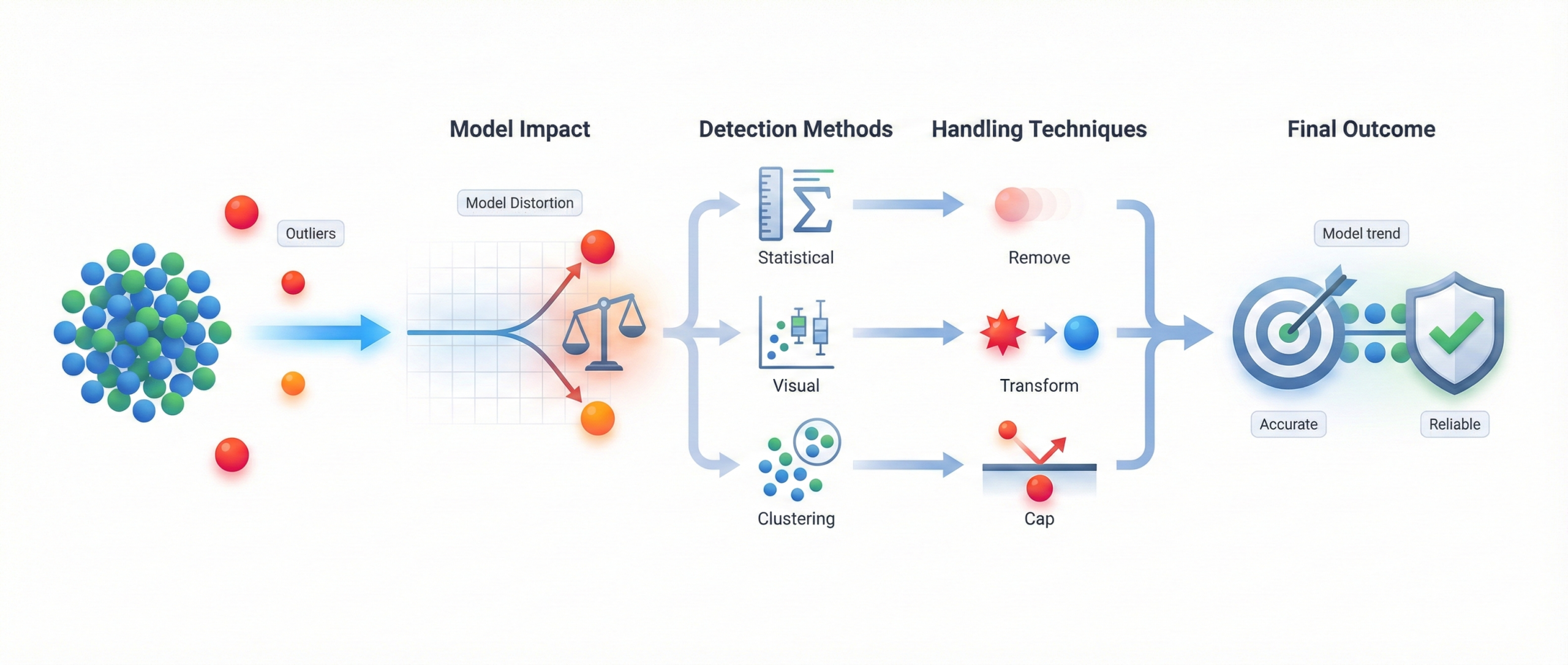
Outliers are data points that deviate significantly from
the normal pattern of a dataset. If left untreated, they can heavily
influence model behavior and lead to misleading results.
Why outliers matter:
- Can distort model parameters and skew predictions
- Have a strong impact on algorithms like linear regression
- May indicate data errors, rare events, or genuine anomalies
- Can reduce overall model accuracy if ignored
Common detection and handling methods:
- Statistical techniques (IQR, Z-score)
- Visual methods (box plots, scatter plots)
- Clustering or distance-based approaches
- Removing, transforming, or capping extreme values
Real-life example:
In salary prediction, most employees may earn between ₹20,000 and ₹1,00,000
per month, but a CEO’s salary of ₹50,00,000 appears as an outlier.
Including this value can skew the model and inflate predictions.
Properly handling such outliers leads to more realistic and reliable results.
Explain the role of the cost function in machine learning.
The cost function (also called loss function) plays a central
role in machine learning by measuring how far a model’s predictions are
from the actual target values. It provides a clear numerical signal that
guides the learning process.
Key roles of the cost function:
- Quantifies prediction error during training
- Guides optimization algorithms toward better solutions
- Helps adjust model parameters in the right direction
- Directly influences convergence speed and stability
- Determines how well the model performs on unseen data
Common cost functions by task:
- Mean Squared Error (MSE) for regression problems
- Cross-entropy loss for classification tasks
Real-life example:
In house price prediction, if a model predicts a house value far from
the actual selling price, the cost function assigns a high error.
During training, the algorithm adjusts the model to reduce this error.
Over time, minimizing the cost function leads to more accurate price
predictions for new houses.
What is dimensionality reduction, and when should it be used?
Dimensionality reduction is a data preprocessing technique
used to reduce the number of input features while preserving the most
important information in a dataset. It helps models focus on what truly
matters instead of being distracted by noise.
Why dimensionality reduction is used:
- Removes redundant and irrelevant features
- Simplifies complex machine learning models
- Speeds up training and reduces computation cost
- Lowers the risk of overfitting
- Makes high-dimensional data easier to visualize
Popular techniques such as PCA and t-SNE
uncover the underlying structure in high-dimensional data by projecting it
into fewer dimensions without losing key patterns.
Real-life example:
In facial recognition systems, a single image may contain thousands of
pixel values. Dimensionality reduction compresses this information into
a smaller set of meaningful features, allowing the system to recognize
faces faster and more accurately without processing every pixel.
What is the purpose of a confusion matrix?
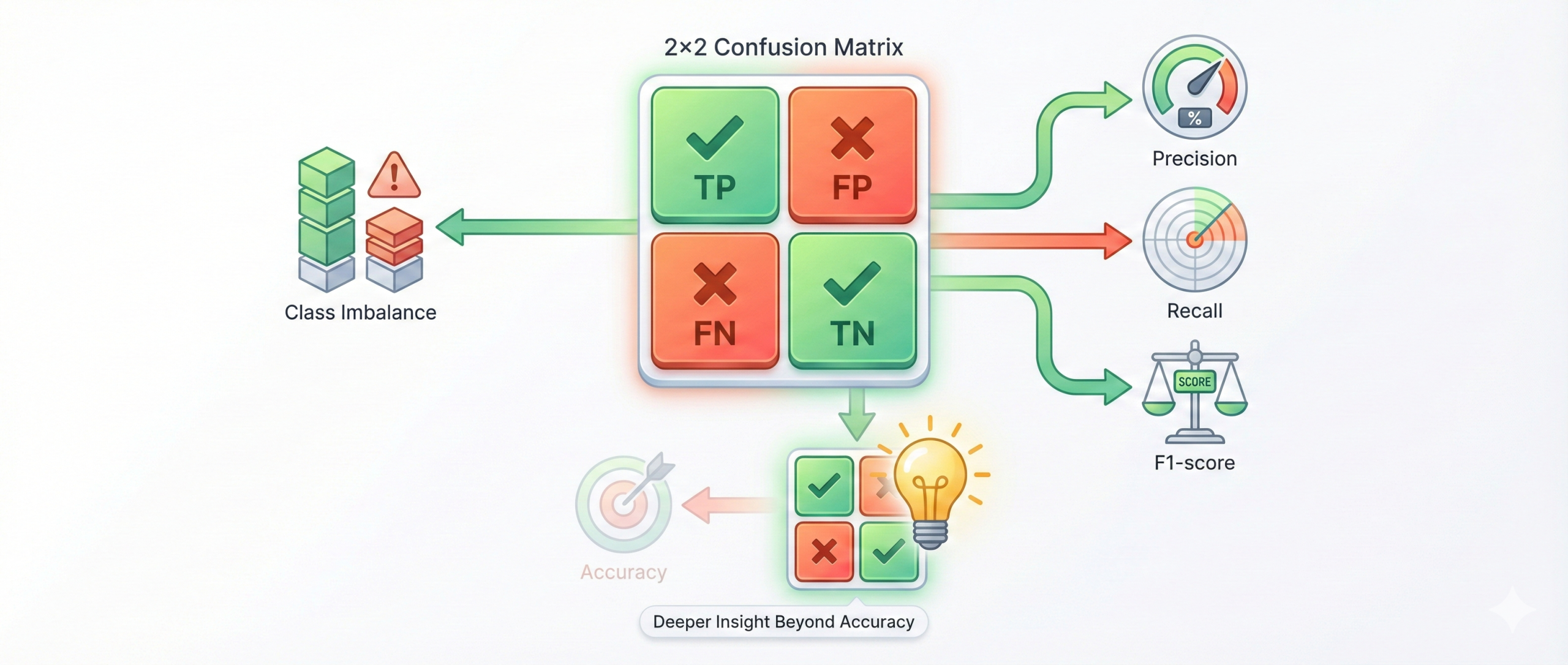
A confusion matrix is a performance evaluation tool used
in classification problems. It provides a detailed breakdown of correct
and incorrect predictions, helping us understand how well a model is
truly performing.
What a confusion matrix shows:
- True Positives (TP) – correct positive predictions
- False Positives (FP) – incorrect positive predictions
- True Negatives (TN) – correct negative predictions
- False Negatives (FN) – missed positive cases
Why it is important:
- Gives deeper insight than simple accuracy
- Helps calculate precision, recall, and F1-score
- Identifies weaknesses like class imbalance
- Helps compare and improve classification models
Real-life example:
In medical diagnosis, a confusion matrix helps evaluate a disease detection
system. Predicting a sick patient as healthy (false negative) can be dangerous,
while predicting a healthy patient as sick (false positive) causes unnecessary
stress. The confusion matrix highlights these errors clearly, allowing doctors
to choose safer and more reliable models.
How does logistic regression perform classification?
Logistic regression is a supervised machine learning algorithm
mainly used for binary classification problems. Instead of predicting
continuous values, it estimates the probability that an input belongs
to a particular class.
How logistic regression works:
- Uses the sigmoid function to convert predictions into probabilities
- Outputs values between 0 and 1, representing class likelihood
- Applies a threshold (commonly 0.5) to decide class labels
- Creates a linear decision boundary between classes
- Trains parameters using maximum likelihood estimation
Why logistic regression is useful:
- Simple and fast to train
- Works well for linearly separable data
- Produces interpretable probability outputs
- Commonly used as a strong baseline model
Real-life example:
In email spam detection, logistic regression predicts the probability
that an email is spam based on features like keywords and sender details.
If the predicted probability crosses a set threshold, the email is marked
as spam; otherwise, it is delivered to the inbox.
What is the purpose of evaluation metrics beyond accuracy?
The purpose of using evaluation metrics beyond accuracy
is to gain a deeper and more realistic understanding of a model’s
performance, especially in real-world scenarios where data is often
imbalanced.
Why accuracy alone is not enough:
- Can be misleading when one class dominates the dataset
- Does not reveal how many errors are false positives or false negatives
- Fails to capture the cost of different types of mistakes
Important evaluation metrics and their role:
- Precision measures how many predicted positives are actually correct
- Recall shows how many actual positives were successfully identified
- F1-score balances precision and recall into a single metric
- ROC-AUC evaluates model performance across different thresholds
Real-life example:
In fraud detection, most transactions are legitimate. A model that labels
everything as non-fraud may achieve high accuracy but completely fail
to catch fraud cases. Metrics like recall and ROC-AUC reveal whether the
model is actually identifying fraudulent transactions, which is far more
important for business safety.
What is the ML pipeline, and why is it important?
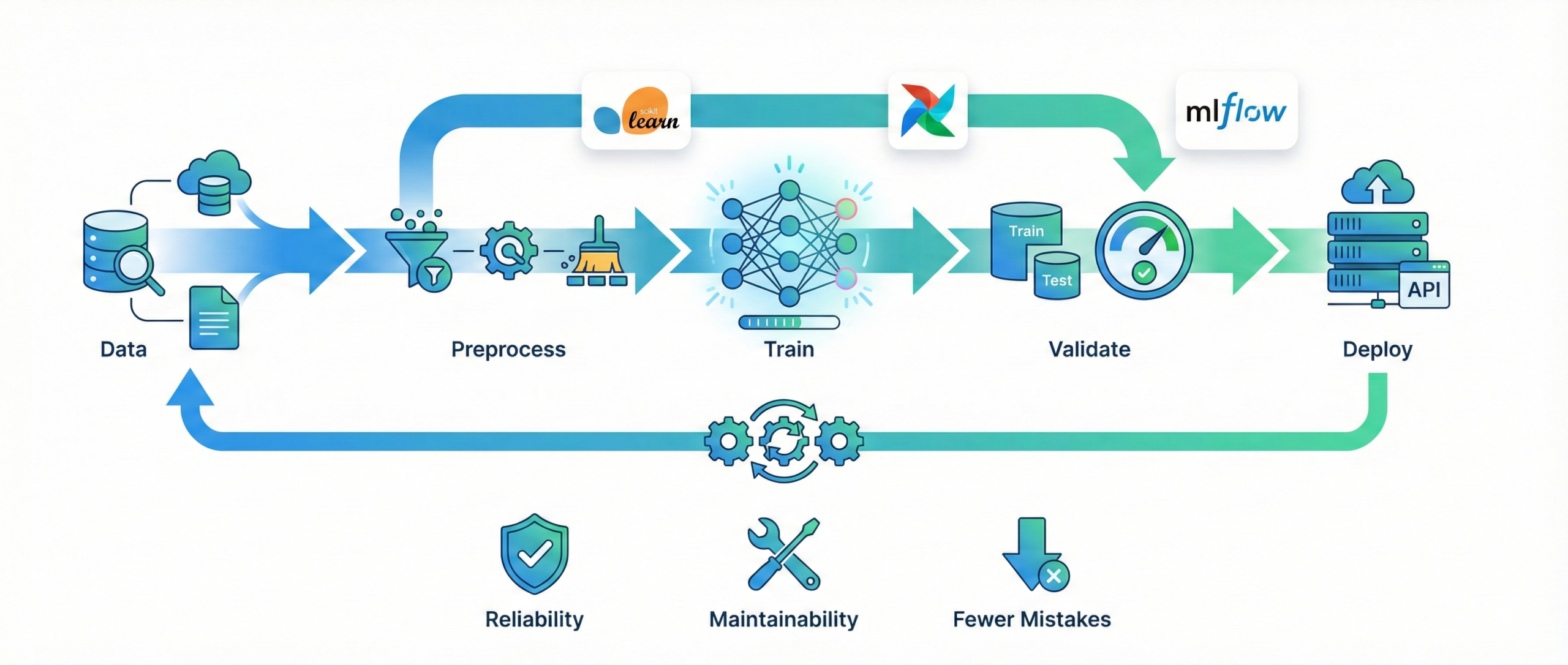
An ML pipeline is a structured workflow that automates the
complete machine learning process, from raw data handling to model deployment.
It ensures that every step is executed in the correct order without manual
intervention.
Key components of an ML pipeline:
- Data loading and ingestion
- Data preprocessing and feature transformation
- Model training and validation
- Performance evaluation
- Model deployment and monitoring
Why ML pipelines are important:
- Ensure reproducibility and consistency across experiments
- Reduce manual errors in large data workflows
- Apply transformations in the correct sequence
- Make models easier to update, retrain, and maintain
Common tools used:
- Scikit-Learn pipelines for model building
- Apache Airflow for workflow scheduling
- MLflow for experiment tracking and deployment
Real-life example:
In an e-commerce recommendation system, new user data arrives daily.
An ML pipeline automatically cleans the data, updates features,
retrains the recommendation model, validates performance, and deploys
the improved version without disrupting users. This automation keeps
recommendations accurate and reliable over time.
What is the purpose of hyperparameter tuning?
The purpose of hyperparameter tuning is to find the best
configuration of a machine learning model so that it delivers the highest
possible performance on unseen data. These settings are defined before
training and strongly influence how a model learns.
Why hyperparameter tuning is important:
- Helps identify the most effective model configuration
- Improves accuracy and overall predictive performance
- Reduces overfitting by controlling model complexity
- Ensures better generalization to new, unseen data
- Is a critical step before deploying ML systems
Common hyperparameter tuning methods:
- Grid search – tests all combinations systematically
- Random search – explores random parameter values
- Bayesian optimization – uses past results to guide future searches
Real-life example:
In a recommendation system, choosing the wrong learning rate may cause the
model to learn too slowly or become unstable. Hyperparameter tuning helps
find the right balance so recommendations improve steadily and remain reliable
for users in real-world usage.


